This model is based on that published in Singh, R., Eliasmith, C. (2006). Higher-dimensional neurons explain the tuning and dynamics of working memory cells. Journal of Neuroscience. 26, 3667--3678. [pdf]
-
To run this demo, open somatosensory working memory.nef.
-
Once it's loaded, run it for 3s by right-clicking the Network Viewer.
-
One interesting aspect of this model is that it uses adapting neurons (spike rates change with constant input).
-
The far more interesting thing about this model is that it explains the data set from Romo et al. (1999) on somatosensory descrimination task in the macaque. The classes of neural response that they indentified is shown in figure 1. No other model has been able to capture all of these response types.
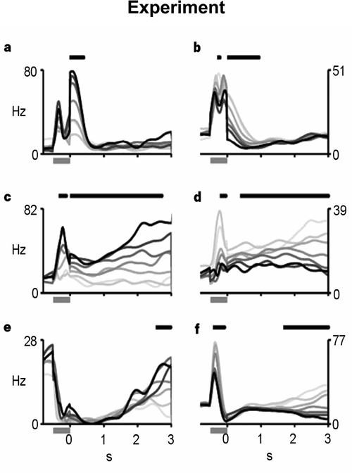
Figure 1: PSTH plots during memorization. The gray bars under the axes indicate the onset of the stimulus, and black bars above the graph mark periods of monotonicity. The higher stimulus frequency (f1) is marked with darker response curves. a, c, e, Positive monotonic. b, d, f, Negative monotonic. a, b, Early neurons. c, d, Persistent neurons. e, f, Late neurons. [Graph from Romo et al. (1999).]
-
To compare the model, you can open the Spike Pattern in the Data Viewer for the somatosensory cortex population. Note that the data above is filtered with a Gaussian kernel to make it into smooth firing rates, you will have to compare spike densities.
-
Look to see if you can find the classes of neuron experimentally identified above in the spike raster.
- For instance 'c' above has some neurons with a brief initial burst and then reasonably constant firing.
- As well, some neurons have very rapid bursts and then silence ('b'), or prolonged silence until a later increase in firing ('e'). Few neurons slow down firing over time (some lines in 'd').
- To verify that the full set of patterns is present, you have to run the simulation with a variety of inputs, and track a single neuron across different inputs.