Neural integrators are often used in sensorimotor systems, with perhaps the best known example being eye control. However, they are also important for path integration, optimal inferencing, noise supression, working memory, and many other biologically relevant computations. Integrators essentially extend the time constant of their elements (neurons) by using recurrent feedback. We can show that for a neural ensemble to approximate integration, it needs to connect to itself with an identity transformation (i.e. x = Ix), and have an input weight of τ, which is the synaptic time constant of the neurotransmitter used on the input. This integrator model can be directly loaded by opening neural integrator.nef within Nengo. Alternatively, follow these steps to build it yourself. 1. Create a one- dimensional ensemble called Integrator with 225 neurons. - From the file menu, select New Network and provide the name Integrator - Right-click on the background of the network window and select Create new->NEFEnsemble - Enter the parameters: 225 neurons, radius of 1, dimension of 1. 2. Add two terminations with synaptic time constants of 0.01s. Call the first one input and give it a weight of 0.01. Call the second one feedback and give it a weight of 1. - Right-click on the ensemble and select Add decoded termination - Enter the parameters above. For the weight, set the input dimension to 1 and click on Set weights to enter the value. - Repeat for the second termination (feedback) 3. Create a new Function input using a Constant Function with a value of 1. - Right-click on the background of the Network Viewer and select Create new->Function Input - Click Set functions and choose or set the appropriate values 4. Connect the network - Connect the Function input origin to the input termination by dragging - Connect the X origin of the ensemble back to its own feedback termination by dragging 5. Gather data - Right-click the population and select Add probe->X - Function of NEFEnsemble state - Right-click the population and select Collect spikes to gather a spike raster - You can add any other probes of interest, including on individual neurons. You see the neurons by double-clicking the population. 6. Run the simulation 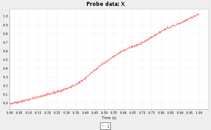- Right-click on the background and run the simulation for 1 second with a time step of 1ms (0.001) - Plot the results by double-clicking the probe of interest in the Data Viewer. - As expected, the final result of the representation in the X probe is approximately 1 (the integral of 1 from 0 to 1). - To adjust the input in real time, right-click on the background and select Interactive plots. Open plots by right-clicking on the objects and add a control slider by right- clicking on the function input. All items can be moved and resized by dragging. See the interactive plots reference sheet. Congratulations, you're done! The remainder of the tutorial demonstrates variations on the basic integrator. ## Representation Range - Run the simulation again, but adjust the end time to be 2.0s. - Note that the value reaches slightly above 1 and then stops increasing. This is due to the radius of the ensemble: it cannot accurately represent values outside of [-1,1] because the neurons are saturating. - Adjust the radius of the ensemble to 1.5 using either the Configure interface (right-click the integrator and select configure, then change the radii option) or the script console (View->Toggle script console, select the population and type that.radii=[1.5] into the console). Run the model again and it integrates longer before saturating. 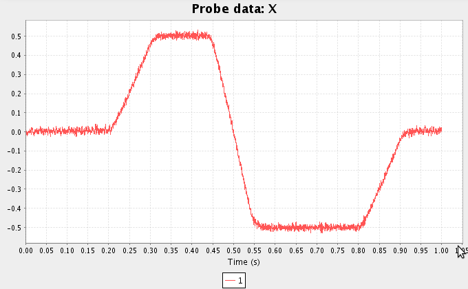## More interesting input - We can also run the model with a more complex input. Change the Function input using the following command from the script console (after clicking on the function input) that.functions=[PiecewiseConstantFunction([0 .2,0.3,0.5,0.6,0.8,0.9],[0,5,0,-10,0,5,0])] - Run this simulation for 1s. ## Changing the number of neurons & synaptic time constants - Note that there may be a significant amount of drift in the representation. This can be reduced by increasing the number of neurons. This can be done in the configure menu (right-click the integrator, and select configure). Double-click neurons and enter the number you'd like. WARNING: values much over 1000 may be slow to generate, although you can run simulations of millions of neurons on workstations. - You can also reduce drift by using a different neurotransmitter. - Change the input termination to have a tau of 0.1 (100ms: NMDA) and a transform of 0.1. Also change the feedback termination to have a tau of 0.1 (but leave its transform at 1). This can be done by right-clicking the termination and selecting configure.