In parts 1 & 2 of this tutorial we determined how to construct a network to perform arbitrary linear transformations, and nonlinear transformations of one variable. In part 3, we extend this to compute nonlinear transformations of any number of variables.

1. Construct the needed populations

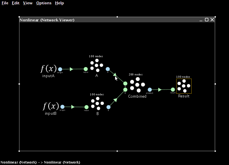
2. In a clean Nengo world right-click and select New network. Construct three populations of neurons (NEFEnsembles), A, B and Z, that are 1 dimensional with 100 neurons each. A and B should have a radius of 10 and Z should have a radius of 100. The radius is the range these neurons are optimized to represent.

3. Construct an H population with 2 dimensions, 200 neurons, and a radius of 10.

4. Add input functions

5. Create two Constant input functions with 1 dimension each and values of 8 and 5.

6. Add terminations to the populations

7. Add input terminations to A, B, and Z with time constants of 0.01 (AMPA) and a weight of 1.

8. Add two input terminations to the hidden layer, H. For each one, the input dimension is 1. For the A input, use Set Weights to make the transformation be [1 0]. For the B input, use Set Weights to make the transformation be [0 1].

9. Create the nonlinear origin

10. Now we need to create a new origin that will estimate the nonlinear function between the two values stored in the H ensemble. For this example we'll just compute the product.

11. Right-click on the H ensemble and select Add decoded origin. Set the name to product. Set Output dimensions to 1.
12. Click on Set Functions. Select User-defined Function and press Set. For the Expression, enter x0*x1.

13. Press OK, OK, and OK to finish creating the origin.

14. Connect the network

15. Connect the two function inputs to A and B, respectively.

16. Connect A and B to the appropriate H terminations.

17. Connect the product origin of H to Z.

18. Collect data and run the simulation

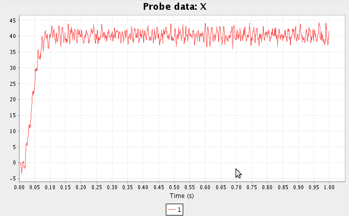
19. Add a probe to the Z ensemble by right-clicking on it and selecting Add probe-> X - Function of NEFEnsemble state. Run the simulation.

20. The result should be approximately 40.
21. Performance can be improved by increasing the number of neurons in the ensembles. The number of neurons can be adjusted using the Configure option (right-click on the ensemble) or the script console (click on the ensemble to select it and then open the console and enter that.neurons=200).
    • WARNING: large numbers of neurons (>500) can take a long time to calculate.
    • This graph uses 500 neurons for the one-dimensional ensembles and 1000 for the combined ensemble
22. Interact with the network by right-clicking and choosing Interactive plots. In this new window, right-click to show controls for changing the input and live plots of spikes, decoded values, voltages, etc. See the interactive plots reference sheet.

Congratulations you can build nonlinear brains!

By combining the two parts of this tutorial, you can build neural models that (attempt to) compute any linear or nonlinear function of arbitrarily high- dimensional vectors. Of course, these are feedforward only. For examples of recurrent models, see the linear neural integrator and nonlinear controlled integrator tutorials.