This tutorial assumes you have completed (or at least read through) the Building a neural integrator tutorial.
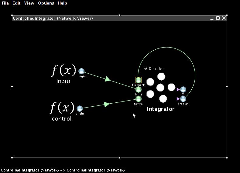
The controlled integrator is a more sophisticated computation, that implements a nonlinear dynamical system. It essentially allows the inputs to control how much integration the network performs, on-the-fly. It can be thought of as a tunable low-pass filter. This model can be directly loaded by opening controlled integrator.nef within Nengo, or you can build it yourself by following these steps.
-
Create a 2-dimensional neural ensemble with 500 neurons and a radius of 2.
-
Create three terminations
-
input: time constant of
0.05, dimension 0f1, transformation matrix of[0.5 0]. This acts the same as the input in the previous model, but only affects the first dimension. - control: time constant of
0.01, dimension of1, with a transformation matrix of[0 1]. This stores the input control signal into the second dimension of the ensemble. Note that it uses a faster time constant, since we want to be able to tune the filter quickly. -
feedback: time constant of
0.05, dimension of1, with a transformation matrix of[1 0]. This will be used in the same manner as the feedback termination in the previous model. -
Create a new origin that multiplies the values in the vector together
- Right-click on the population and select Add decoded origin
-
This is a
1dimensional output, with a User-defined Function ofx0*x1(this effectively multiplies the first and second inputs, hence allowing one to control/gate the other). Note that no actual multiplication occurs in the neurons, instead this is a projection from a two-dimensional to a one-dimensional space. This may take a moment to configure. -
Create two Function inputs called input and control.
-
Start with Constant functions with a value of
1 - Use the script console to set the input function by clicking on it and entering the following input function.
that.functions=[ PiecewiseConstantFunction( [0.2,0.3,0.44,0.54,1.3,1.7] ,
[0,0.5,0,-1.0,0,0.5,0 ])]
-
Use the script console to set the control function by clicking on it and entering
that.functions=[ PiecewiseConstantFunction( [0.9] , [1,0.5] )] -
Connect the network
-
Connect the input function to the input termination, the control function to the control termination, and the product origin to the feedback termination.
-
Run the simulation and plot results as before
-
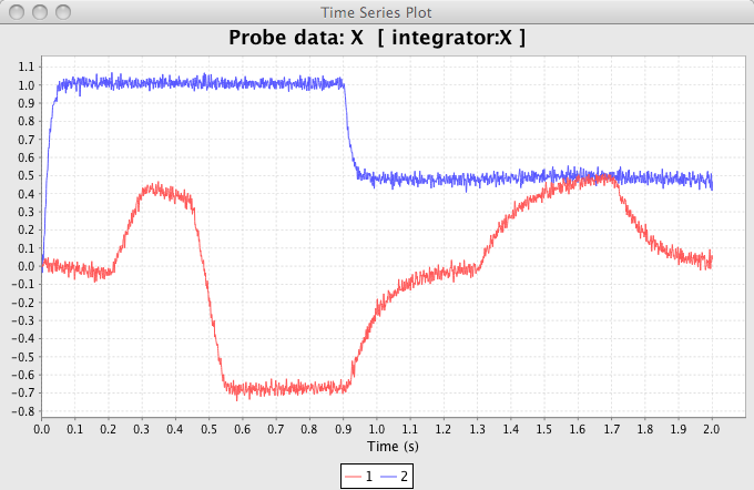
Add a probe to the X representation of the integrator and the origin of the function input
- Run the simulation for 2s. Plot X. If you select both the input and integrator data (via Ctrl-clicking) and plot them together through the right-click menu, they will be on the same graph.
-
For the first 0.9 seconds, the network will act as an integrator (a control signal of 1). After this, the control signal will drop to 0.5, which will cause it to act as a highly leaky integrator, or a low-pass filter.
-
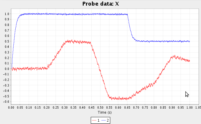
We can improve the performance of this model by increasing the number of neurons. On the right it is run with 5000 neurons in the ensemble for 1s.
- WARNING: 5000 neurons take a long time to generate (~5 minutes) on a good laptop.
- You can also run the simulation interactively: right-click the background and select Interactive plots. See the interactive plots reference sheet.