In this tutorial, you will connect groups of neurons to control a robot moving around its environment. The robot has two range sensors and two motors, so you will use the standard Braitenberg Vehicle control system.

1. Create the robot and its world

2. Open the Script Console by going to View->Toggle Script Console.

3. Type run NIPSDemos/vehicle.py. Wait a moment for the network to be created.

4. Run the Simulation

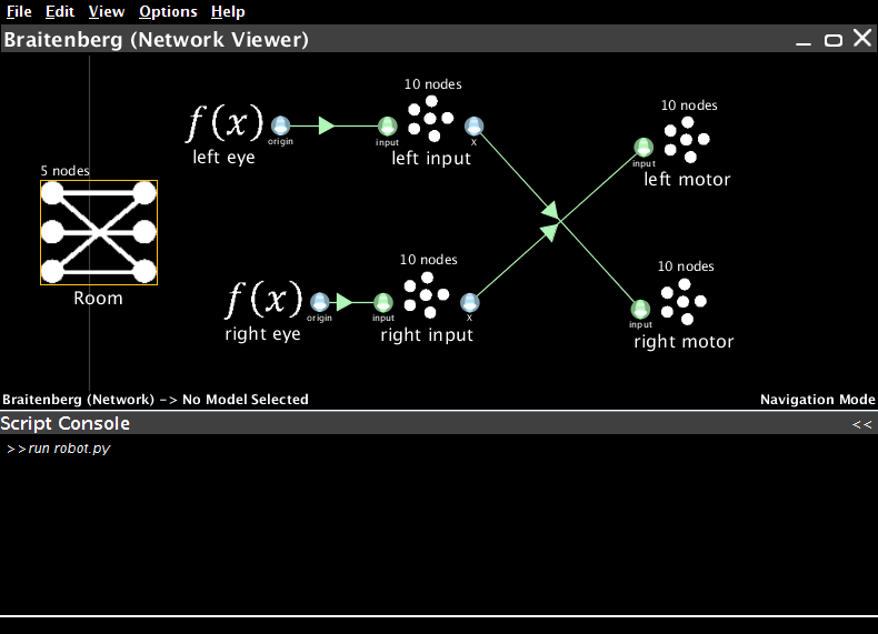
5. Open the Network Viewer by double-clicking on the Braitenberg network

6. Right-click inside the Network Viewer and select Interactive plots
7. Press the play button (bottom right).
8. The graphs show the spike rasters from four groups of neurons: two groups of afferent sensory neurons; and two groups of efferent motor neurons. Next to these is the graph of the decoded values from these spikes.
9. Boxes will fall, but the robot will not move because its inputs have not yet been connected to its motors.

1. Connect the network

2. Go back to the Network Viewer

3. Click on the left input's origin called X and drag it to the right motor's termination. This will connect the two, calculating the optimal synaptic connection weights to transfer information between neural populations.

4. Do the same to connect the right input to the left motor.

5. Run the Simulation

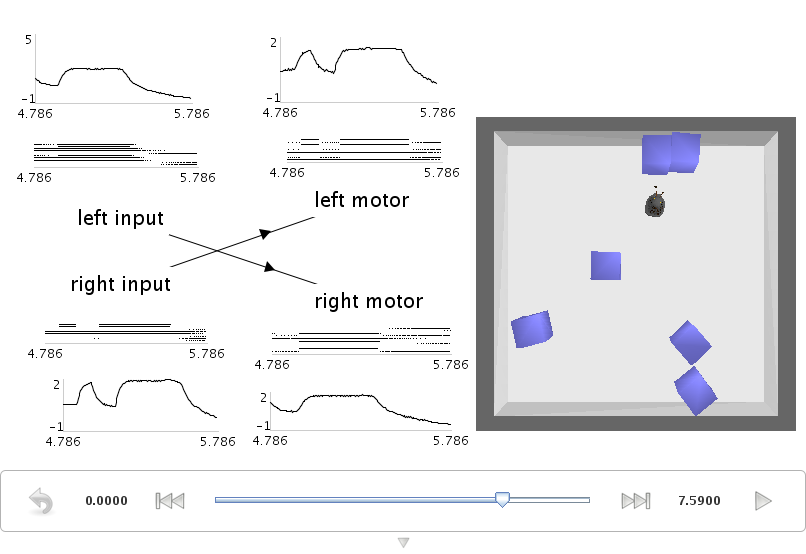
• Go back to Interactive plots.
• The robot should be attempting to avoid walls.
• Reset the simulation (by pressing the arrow in the bottom left) if the robot seems stuck.
• Since the left sensor is connected to the right motor, notice that the value graphs for these two neural groups are similar. However, the spike rasters will be quite different. Some neurons fire more for large values, while other fire more for small values.
• What happens if you connect the inputs the other way around? Try this and see the change in the robot's behaviour. You can connect and disconnect the neural projections while the simulation is running.