This tutorial assumes you've completed Building a feedforward network (part 1).
Scaling the input signal
-
Right-click on the input to the B population and select Configure.
-
At the bottom of this panel double-click transform. This is the weight you set to 1 when constructing the termination. Change this value to
0.5to scale the input down to half its original value. -
Re-run the simulation (or go to interactive plots), and see that changing this value scales the input as expected.
Combining inputs linearly
 To add two values, you must create another
termination on the B population and project to it as well. Before doing
this, set the A to B transformation back to 1.
-
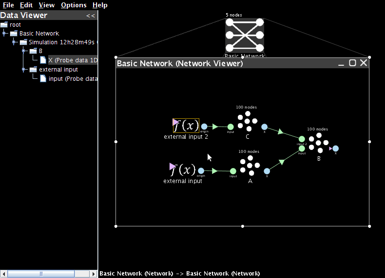
Create a termination on the B population called
input 2with weight1. -
Create a new ensemble C.
-
Create a projection from C's X origin to input 2 by dragging.
-
Create a new constant Function input and set its value to
-0.7. -
Add an input termination on C and connect the Function input to the C ensemble.
- Add a probe to the new Function input.
- Run the simulation and plot the values for the three probes

- The X value for the B probe should indicate the result of
0.5-0.7=-0.2(A+C=B). Note: This looks noisier than before because of the scale of the plot.
Congratulations, you can build linear brains!
You can now compute any linear transformation in a neural circuit. Exactly the same steps as above can be followed for vector representations, where the transformation weight becomes a matrix. For more on vector representation, see the motor cortex tutorial.
Nonlinear transformations
Of course, nonlinearities are essential for interesting computation. We begin with simple examples here before moving on to more interesting examples in part 3.
-
Revert the simulation to a communication channel
-
Right-click on the C population and select remove model. Answer Yes to delete the population.
-
Do the same to the the second Function input and the input 2 termination on the B population (right-click just on the termination).
-
Define the nonlinear function you want to compute
-
For one-dimensional ensembles, we can calculate arbitrary 1-dimensional functions (e.g. f(x)=x2, f(x)=θ(x) (thresholding); f(x)=√x, etc.).
- To perform a non-linear operation, we need to define a new origin. Right-click on the B ensemble and select Add decoded origin. Set the name to
squareand dimension to1. - Click on Set Functions, select User-defined Function and press Set.
-
For the Expression, enter
x0*x0. We refer to the represented value asx0. When when have vectors the values arex0,x1,x2, etc. Press Ok, Ok, and Ok. -
Collect data from the new output
-
Add a probe for the new origin by right-clicking on the ensemble and selecting Add probe->square - Function of NEFEnsemble state
-
Set the input function to something useful
-
Click on the input function that is currently a constant value. You can change this in two ways, through the configure panel or the script console. Let's do the second for variety.

- Open the Script Console from the menu bar (under View).
- With the function input selected type the following in the console:
that.functions=[InterpolatedFunction([0,1],[-1,1])]
-
This creates an input that starts at -1 and grows linearly to 1
-
Run the model and view the probe data. The output of the network will approximate x2. Note that there is an initial start-up transient in the graph (shown above). You can also use the Interactive plots to manually control the input. See the interactive plots reference sheet.