In this demo you simulate a network that learns nonlinear feedforward transformations of a scalar. Variants of this network will learn dynamic (recurrent) transformations as well vector transformations. We do not discuss these extensions here.
For those online, all of the files needed for this simulation are in learning
scalars.zip. Be sure to place the
learning_rule.py file in the python
directory.
- Open the network to be simulated.
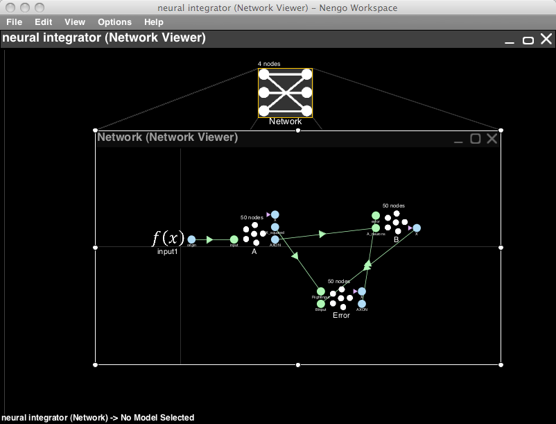
- On a blank Nengo world, got to File->Open from file the menu bar. Select learning scalars.nef and click Open.
-
(Skip this step if you don't care about scripts) This network was generated from the learning_scalars.py script. To view the script select View->Open script editor. In the editor select File->Open and open the file learning_scalars.py. To run the script to generate this network, open the script console (View->Toggle script console) and type
run NIPSdemos/learning_scalars.py. -
Run the network
-
You can run the network as is for 2s by right-clicking in the Network Viewer.
-
Look at the graphs by expanding the tree in the Data Viewer. (The default input is Gaussian white noise)
-
Interact with the network
-
Instead of looking in the Data Viewer you can interact directly with the network.
- Right-click in the Network Viewer and select Interactive plots
- Hit the play button (bottom right). The network will be injected with Gaussian white noise, and begin to learn the nonlinear transformation defined (x2).
- You can plot spiking behaviour, etc. as desired. See the interactive plots reference sheet.
- Note that the network learns reasonably quickly. After the first few seconds it is able to perform the defined nonlinearity reasonably well. This is evident from the lessening of the error, and the graph from the B population compared to the graph from the A population (or the input).
-
Note also, that if you reset the network, it does not re-initialize the weights to a random matrix. You have to reload the .nef file to do that. So hitting play after reset will use already learned weights.
-
Change the learned function
-
Close the interactive plots
- Drag the connection from to the RightInput on the error population away from the population (so it disconnects, but don't remove it).
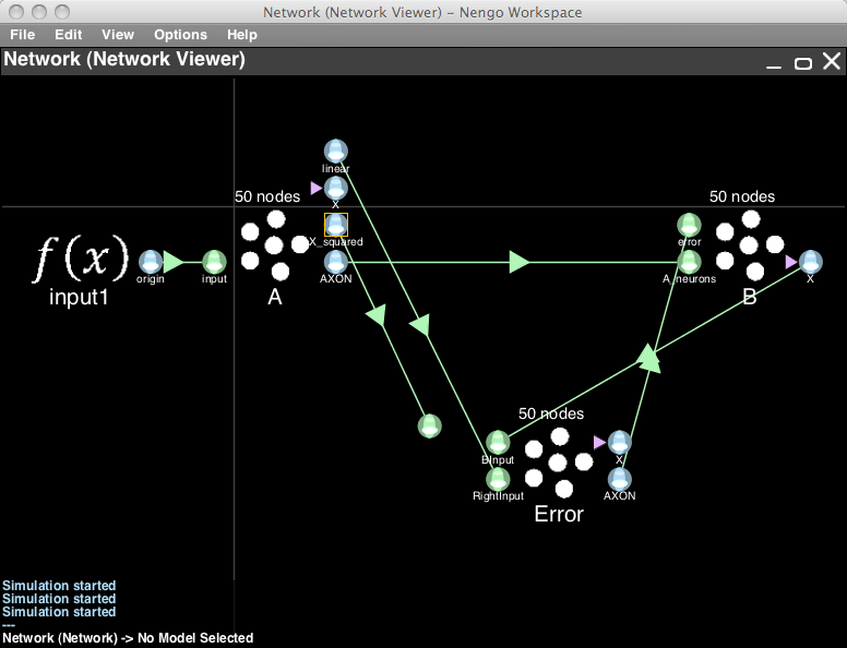
- Right-click A and select Add decoded origin. Click Set functions, choose User defined function, click Set, and you can type a function in terms of the represented variable
x0. A simple linear function is0.5*x0, which is just a scaled version of the input. - Connect your new origin to where you disconnected the previous origin. Re-open the Interactive plots and watch the system attempt to learn the newly defined function.
- You can now switch the connections while the simulation is running. Drag the new origin connection off, and the x_squared connection back on to the RightInput termination. You will see the effects immediately in the plots.
- This experiment shows that the weights that are learned between A and B are the weights that subtract the error from the defined function (if you remove the error connection to the B population, you will see the system break down slowly).