In part 1 of this tutorial we will build an extremely simple circuit in Nengo, which simply communicates a single scalar value from one population of neurons to another (a communication channel). We will then implement linear and nonlinear transformations of that value in a feedforward network in part 2. In part 3, we will look at more complex representations (vectors) and more sophisticated nonlinear transformations.
-
Create two populations of neurons
-
Right-click on the background of the Nengo world and create a New network called
feedforward network. - Right-click inside feedforward network and select create new-> NEFEnsemble.
- Set the name to
A, the number of nodes to100, radius to1, dimension to1, and select LIF Neurons. Click Ok. - Do the same to create a
Bensemble. -
Right-click on either A or B and select Plot->Constant rate responses. This shows the tuning curves of the neurons.
-
Create terminations on the receiving population
-
Connections between ensembles are built using origins and terminations. An origin from one ensemble can be connected to a termination on another.
- Right-click on the B ensemble and select Add decoded termination. Set the name to
input. Set the input dimension to1and click Set weights1`. -
Set tauPSC to
0.01. This synaptic time constant differs according to which neurotransmitter is involved. 10ms is a reasonable time constant for AMPA (5-10ms). -
Connect the populations together
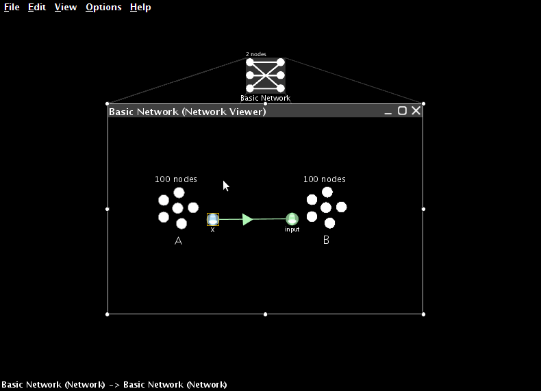
- Every ensemble automatically has an origin called X. This is an origin suitable for building any linear transformation.
-
Click and drag from the X origin from A to the termination on B. This will create the desired projection between the neurons in the populations. This calculates the connection weights between all neurons in both populations necessary to compute the function you have defined (which is B=1*A at the moment).
-
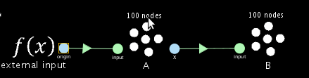
Add an input function to drive the neurons
-
Right-click inside the Network Viewer and choose Create new->Function input. Give it the name
external input. Set its output dimensions to1. - Press Set Function to define the behaviour of this input. Select Constant Function from the drop-down list and then press Set to define the value itself. For this model, set it to
0.05. -
Add a termination on the first neural ensemble A following the steps above and connect the input function to that ensemble by dragging.
-
Collect some data
-
Before running the simulation, we need to identify which aspects of the simulation we want to save for later analysis. The main method for doing this is via Probes. For this case, we will add two probes: one to record from the external input and one to record from the B ensemble.
- Right-click on the external input and select Add probe->input. A triangle will appear indicating the presence of the probe.
- Right-click on the B ensemble and select Add probe->X - Function of NEFEnsemble state.
-
Right-click on the B population and select Collect Spikes to record the neuron spike trains.
-
Run the simulation
-
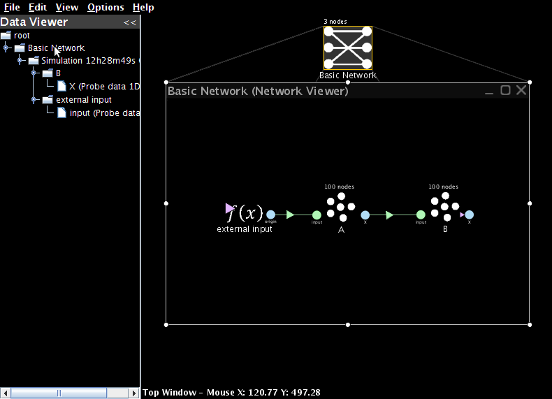
Right-click on the Network Viewer background and choose Run feedforward network
- Set start time to
0, step size to0.001(for a 1ms time step), and end time to1. For convenience, enable the setting to open the data viewer after simulation. Click OK. When finished, the Data Viewer panel will appear on the left. - Expand the Data Viewer tree by clicking on the entries until the two probes are shown
- Double-click Spikes Pattern to see the spikes generated by the neurons.
- Double-click on the input probe to show that the input stays at 0.5 over the whole simulation
- Double-click on the X probe to show what value is encoded by the second neural ensemble over time.
- To compare these plots, select both probes by ctrl-clicking to on the probes in the Data Viewer tree. Now right-click and select Plot data together.
- You can also interact with this model in real time. Right-click on the Network Viewer background and select Interactive plots.
- Press the play button (bottom right) and slide the control up and down. The graph will show the output caused by the changing input. Other plots are available from this screen by right-clicking network elements. See the interactive plots reference sheet for more details.
Congratulations, you're done!
You've finished building a simple neural communication channel. If you want to increase the accuracy, you can increase the number of neurons in the populations (the more neurons you choose, the more patient you will have to be while they are generated). However, brains do more than just represent their input; parts 2 and 3 show how to actually do some transformations.